How to compute the safety stock, Shall I use the demand distribution or the forecast demand error distribution??

Currently, I am teaching a subject about operations management and I have to introduce to my students the importance of safety stocks and the different ways to determine it. At this point, I was analyzing how this issue is explained in operations management books, and I realized that some of them compute the safety stock on the basis of the lead time demand distribution (Heizer and Render,  2008), whereas books more specialized in inventory management (Silver et al, 1998) and (Nahmias, 2004), they suggest to use the lead time forecast demand distribution.  To be more precise, if we compute the safety stock for a certain service level, the safety stock (SS=k*standard deviation of lead time demand), where k can be obtained given the service level. The problem relies on the standard deviation, shall I use the standard deviation of the lead time demand distribution or shall I use the standard deviation of the lead time forecast demand error?

Intuitively, if my product forecasts are accurate I should have less safety stock and if my forecast errors are high, then I should increase the safety stock. Therefore, the safety stock should be computed based on the lead time forecast demand distribution. Nonetheless, I was trying to look for an clearer example, because I was not sure whether my students will be totally convinced with such a justification. The idea is to find an example where the demand distribution had a high variability but the demand forecast provided lower errors… and thinking a little bit… we could imagine a seasonal product. In the particular case of a seasonal product, the demand variability can be high, but the forecast of its demand can be quite precise.

Let’s consider the following example. Suppose that we have two products, the first product demand is the result of a random normal simulation with the following MATLAB code:

%Define time

t=(1:100)’; %100 weeks

%SKU 1

d=normrnd(50,7,100,1); %Demand with mean 50 and standard deviation 7

figure, plot(t,d,‘-k’), ylabel(‘Demand’), xlabel(‘Weeks’), title(‘SKU 1’)

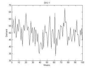
If we run that code, we obtain the following figure:

Figure 1: SKU 1 demand vs. time (weeks).

 

 

 

 

 

Now, we can compute the standard deviation of the lead time demand distribution (let’s asume that the lead time is 1 week for the sake of clarity). In this case, we write in MATLAB

std(d) %compute the standard deviation of the SKU 1 demand.

and the sample standar deviation is 6.7. (Recall that the simulated true estándar deviation was 7).

The second approach is to compute the standard deviation of the lead time forecast demand error. In order to do that, we employ a single exponential smoothing. Note that the data only shows a level + noise, and the exponential smoothing is a good candidate to forecast such kind of data. We can implement that in Matlab as:

f(1)=d(1); % Initialization

alpha=0.02; %Set the value of the constant to 0.02

for i=1:100

f(i+1)=f(i)+alpha*(d(i)-f(i));

end

pred=f(1:100)’;

error1=pred-d, %compute the forecast error

std(error1) %Compute the standard deviation of the forecast error.

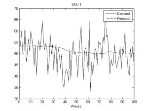
And the standard deviation of the forecast demand error is 6.7 approx. In other words, it is very similar to the standard deviation of the original demand during the lead time. We can also plot the forecast and the real demand, see the following figure:

Figure 2: demand of sku 1 (solid line) and forecast demand of the same sku (dashed line).

 

 

 

 

Therefore, when the data can be modeled as a level + noise, and thus, a single exponential smoothing, or moving averages are adequated to forecasting such a demand, the differences between using the standard deviation of the demand or the forecast demand error are small.

Let’s continue with this example. Now, suppose that the demand follows a seasonal pattern, we can simulate that with the following code:

d2=100*sin(2*pi/10*t)+normrnd(50,1,100,1); % Seasonal period = 10 weeks.

figure

plot(t,d2,‘-k’), ylabel(‘Demand’), xlabel(‘Weeks’),

title(‘SKU 2’)

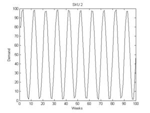
If we run that code, we obtain the following figure:

 

Figure 3: Seasonal demand corresponding to the SKU 2. The seasonal period is 10 weeks.

 

 

 

 

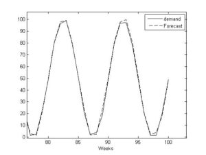
Then, we can compute the SKU 2 lead time demand standard deviation “std(d2)” that provides a value equal to 35.4. Nonetheless, if we forecast such demand with a forecasting technique capable of handling seasonality, for example, the Holt-Winters exponential smoothing (see next Figure to see the forecasts), the standard deviation of the forecasts error are 1.51 (much smaller tan 35.4).

Figure 4: SKU 2 both demand and forecasts (Holt-Winters).

 

 

 

 

 

It should be pointed out that, in this particular case, the demand has a high variability but the forecasts error do not, and if we determine the safety stock with the lead time demand we will be oversizing the safety stock with the consequent costs.

 

In summary, when the data cannot be modeled as level + noise, for example because of seasonal patterns, trend, level-shifts, etc…. It is more adequated to compute the safety stock on the basis of the forecast error lead time demand, otherwise we will be oversizing the safety stock…

Some references:

1. Heizer, J.H and Render B. (2008). “Operations Management”. Pearson Prentice Hall.
2. Silver, E. A., Pyke D. F. and Peterson, R. (1998). “Inventory Management and Production Planning and Scheduling”, Third Edition. John Wiley and Sons.
3. Nahmias, S. (2004). “Production and Operation Analysis”. MacGrawHill